Simulation
The Simulation step evaluates the calibrated parameters on the simulation station and period — data the models were not fitted to. This is where a calibration proves (or fails to prove) that it generalizes: split-sample test when the station is the same and the period differs, proxy-basin test when the station differs.
The step unlocks once calibration has produced parameters, and the result is computed automatically when you open it.
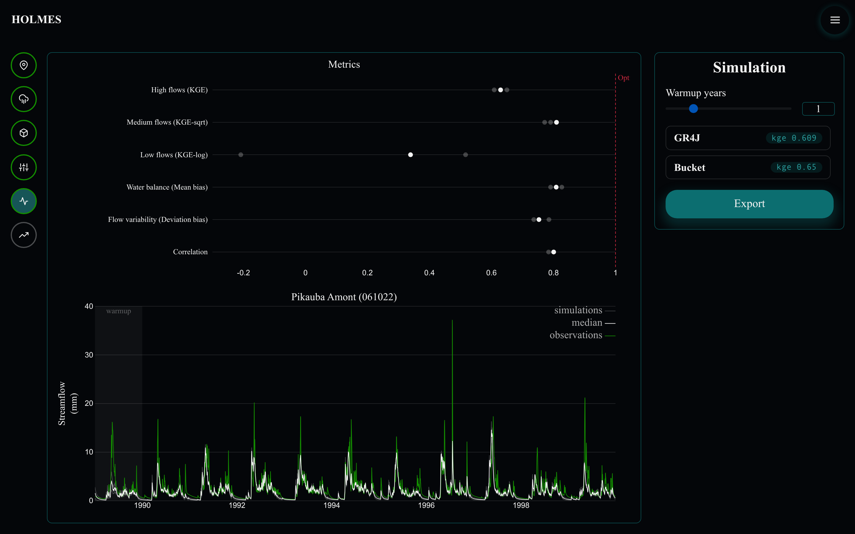
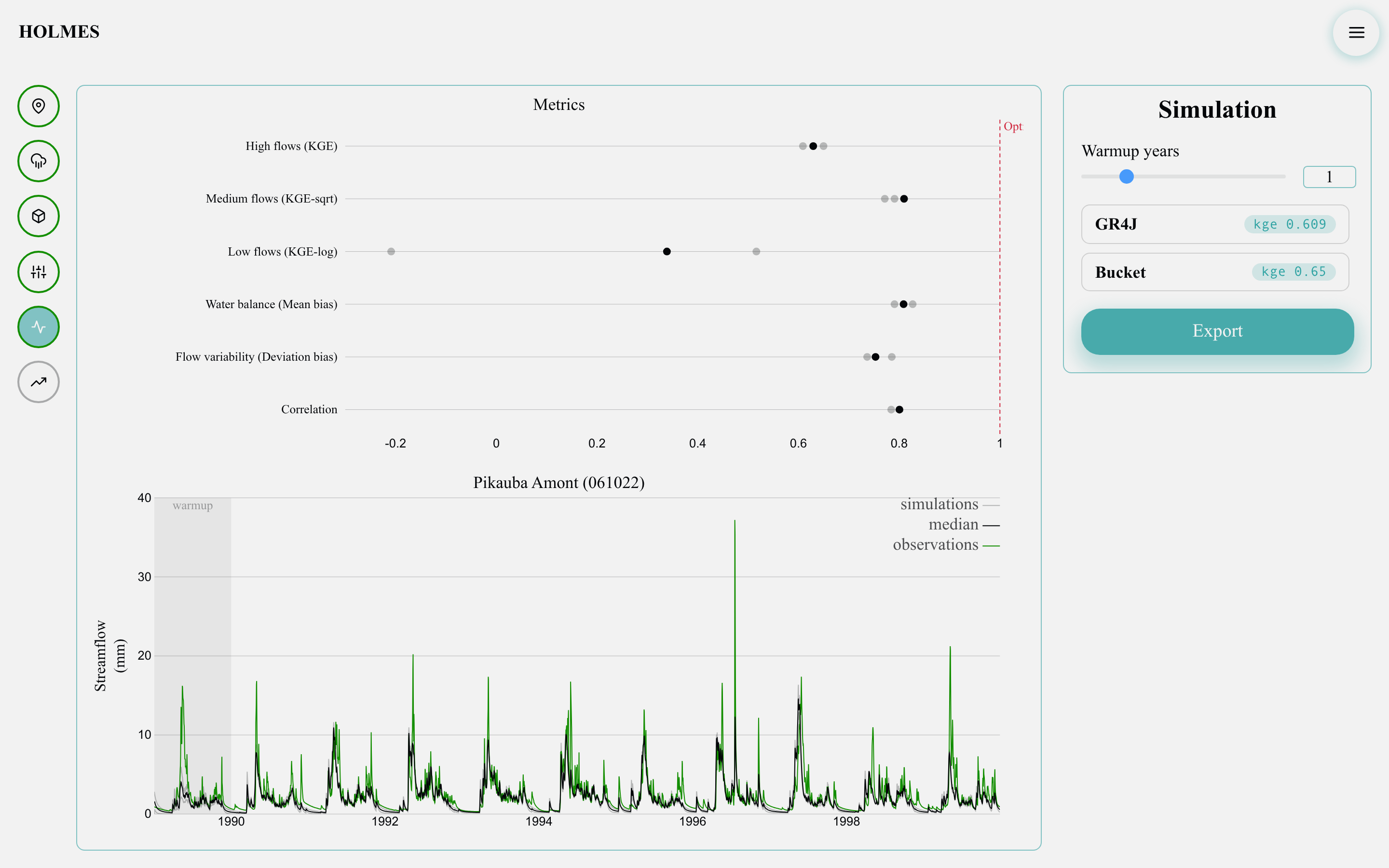
Controls
- "Warmup years" (0–5, default 1) — same role as in calibration: prepended years to spin the stores up, excluded from the metrics.
- One row per model with its KGE over the simulation window; hovering a row highlights that model in both charts.
- "Export" downloads
simulation_<station>_<start>_<end>.json(configuration, each model's parameters and all its metrics) and.csv(datetime,observations,<model…>plusmedianfor ensembles).
The metrics chart
Rather than a single score, the top chart profiles each model's behavior over six metrics, one dot per model plus a solid median dot, against a dashed "Optimal" guide at 1:
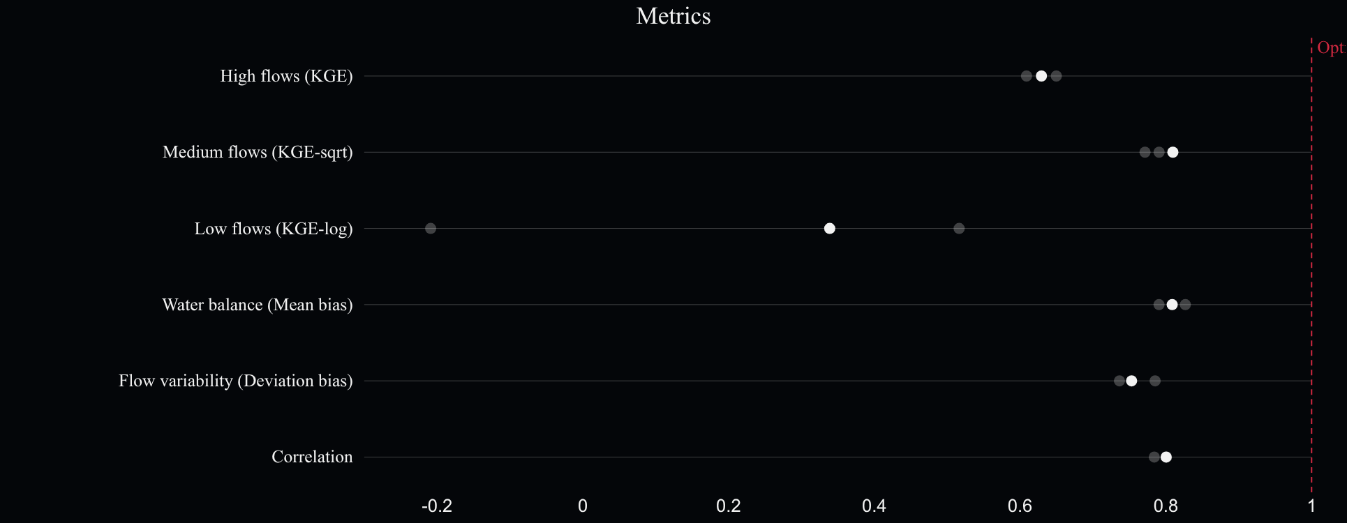
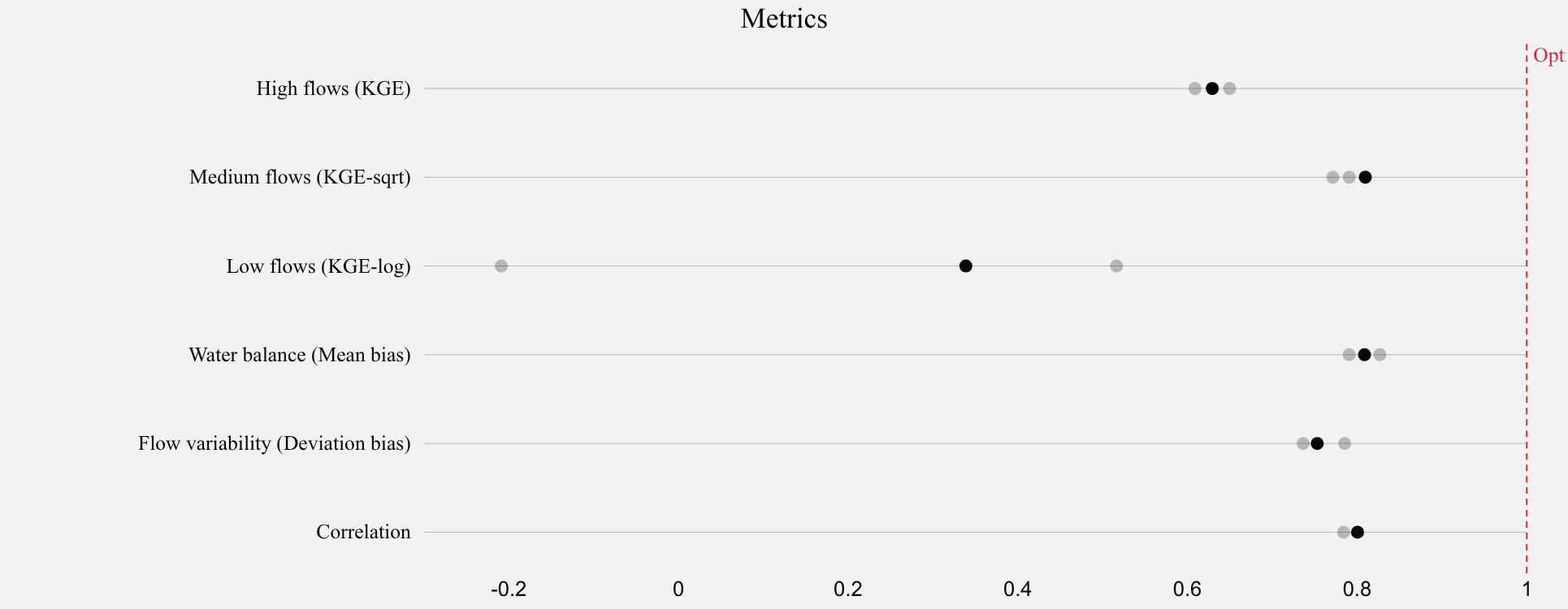
- "High flows (KGE)" — KGE on untransformed flows, dominated by floods;
- "Medium flows (KGE-sqrt)" — KGE on square-root-transformed flows;
- "Low flows (KGE-log)" — KGE on log-transformed flows, dominated by recessions and baseflow;
- "Water balance (Mean bias)" — ratio of simulated to observed mean flow;
- "Flow variability (Deviation bias)" — ratio of the simulated flows' standard deviation to the observed one's;
- "Correlation" — timing of the simulated series against the observations.
A model can score well on floods and still drift on volume or low flows; the profile makes those trade-offs visible at a glance.
The streamflow chart
The bottom chart overlays the observations (green — the simulation station's color) with each model's simulation and the ensemble median, warmup band included.
Simulating outside the observed record
The simulation period may extend beyond the station's record: the models then run on weather alone. The hydrograph still renders, but the metric chips show "kge —" for the days without observations to score against. This is how an unobserved event is reconstructed — for example the July 1996 Saguenay flood at a station whose record only starts later.