Calibration

The Calibration page is where you find optimal model parameters by fitting simulations to observed streamflow data. HOLMES supports both manual parameter adjustment and automatic optimization.

Overview

Calibration is the process of finding model parameters that produce simulated streamflow closely matching observations. HOLMES displays:

• Observed streamflow from the selected catchment
• Simulated streamflow using current parameters
• Performance metrics quantifying the fit

General Settings

The left panel contains configuration options that apply to both manual and automatic calibration.

Hydrological Model

Select the rainfall-runoff model to calibrate:

Model	Parameters
gr4j	4
bucket	6

See Concepts: Models for detailed model descriptions.

Catchment

Select the catchment dataset. Each catchment includes:

• Daily precipitation
• Potential evapotranspiration (PET)
• Observed streamflow
• Optionally: temperature (for snow modeling)

The available date range updates based on the selected catchment.

Snow Model

Enable snow accumulation and melt modeling for catchments with significant snowfall:

Option	Description
none	No snow model (default)
cemaneige	CemaNeige degree-day model

Availability

The snow model option is only enabled for catchments that include temperature data. Catchments without temperature data will show this option as disabled.

Objective Criteria

Choose the metric used to evaluate model performance:

Metric	Optimal	Description
nse	1	Nash-Sutcliffe Efficiency
kge	1	Kling-Gupta Efficiency
rmse	0	Root Mean Square Error

Streamflow Transformation

Apply a transformation to the streamflow before computing the objective:

Transformation	Effect
High flows: none	No transformation - calibrates to match peak flows
Medium flows: sqrt	Square root - balanced emphasis on all flows
Low flows: log	Logarithmic - emphasizes base flow accuracy

Choosing a Transformation

• Use none if flood prediction is your primary goal
• Use sqrt for general-purpose calibration
• Use log if accurate low-flow simulation is critical (e.g., drought studies)

Calibration Period

Set the start and end dates for calibration:

• Dates are constrained to the catchment's data availability
• Click Reset to restore the full available range
• A warm-up period is automatically included before the start date

Warm-up Period

The warm-up period (3 years, or up to the minimum available data) allows model stores to reach realistic levels before the calibration period begins. This period is shown as a shaded area on the chart.

Calibration Algorithm

Choose between manual and automatic calibration:

Algorithm	Use Case
Manual	Learning, exploring parameter sensitivity
Automatic - SCE	Finding optimal parameters efficiently

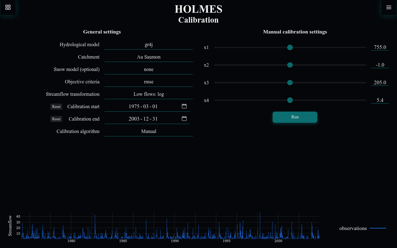
Manual Calibration

Manual calibration lets you adjust parameters directly and see immediate results.

Manual calibration settings

When Manual is selected, parameter sliders appear:

For GR4J:

Parameter	Description
x1	Production store capacity (mm)
x2	Groundwater exchange (mm/day)
x3	Routing store capacity (mm)
x4	Unit hydrograph time base (days)

For Bucket:

Parameter	Description
c_soil	Soil storage capacity (mm)
alpha	Split factor for slow/fast routing
k_r	Slow reservoir recession coefficient
delta	Routing delay (days)
beta	Precipitation split factor
k_t	Fast reservoir recession coefficient

Running a Manual Calibration

1. Adjust parameter sliders to your desired values
2. Click Run to execute the simulation
3. Observe the streamflow chart and objective value
4. Iterate: adjust parameters and run again

Parameter Exploration

Try adjusting one parameter at a time to understand its effect on model behavior. This builds intuition about how the model works.

Automatic Calibration

Automatic calibration uses optimization algorithms to find parameters that maximize (or minimize) the objective function.

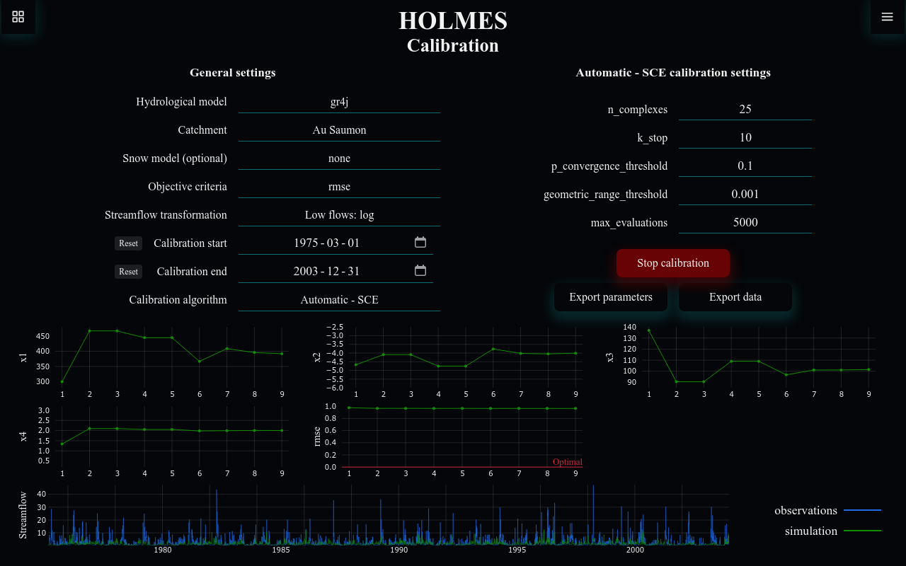
Automatic - SCE calibration settings

When Automatic - SCE is selected, algorithm parameters appear:

Parameter	Description
n_complexes	Number of complexes
max_evaluations	Maximum function evaluations
k_stop	Iterations to check for convergence
p_convergence_threshold	Relative change threshold
geometric_range_threshold	Parameter space convergence

The Shuffled Complex Evolution (SCE-UA) algorithm is a global optimization method well-suited for hydrological model calibration.

Running an Automatic Calibration

1. Configure general settings and algorithm parameters
2. Click Start calibration
3. Watch the real-time updates:
   • Parameter values converging
   • Objective function improving
   • Simulated streamflow matching observations
4. Click Stop calibration to halt early, or wait for completion

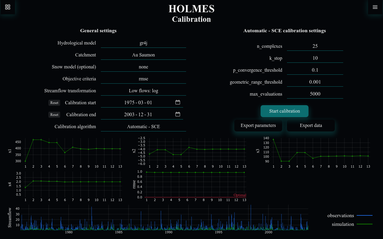
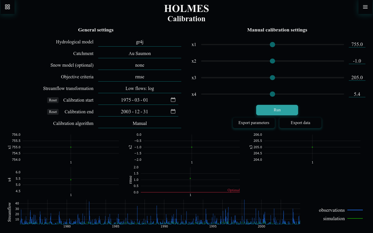
Understanding the Results

During and after calibration, the results panel shows:

Parameter Evolution Charts (one per parameter)

• X-axis: Iteration number
• Y-axis: Parameter value
• Shows how each parameter converges toward optimal

Objective Function Chart

• X-axis: Iteration number
• Y-axis: Objective value (NSE, KGE, or RMSE)
• A horizontal line shows the optimal value (1 for NSE/KGE, 0 for RMSE)

Streamflow Chart

• Blue line: Observed streamflow
• Green line: Simulated streamflow (updates with each iteration)
• Blue shaded area: Warm-up period (excluded from metrics)

Exporting Results

After calibration, export your results using the buttons below the settings:

Export parameters

Saves the calibrated parameters as a JSON file:

{
  "hydroModel": "gr4j",
  "catchment": "Example Catchment",
  "snowModel": null,
  "objective": "nse",
  "transformation": "sqrt",
  "start": "1990-01-01",
  "end": "2000-12-31",
  "hydroParams": {
    "x1": 350.5,
    "x2": 0.12,
    "x3": 95.3,
    "x4": 1.85
  }
}

This file can be imported into the Simulation or Projection pages.

Export data

Saves two files:

1. Calibration results (JSON): Complete parameter evolution and objective values
2. Timeseries data (CSV): Date, observed streamflow, simulated streamflow

Common Issues

Poor Calibration Results

If the objective value is far from optimal:

1. Check that the correct catchment data is loaded
2. Try a different transformation
3. Verify the calibration period includes representative conditions
4. Consider if the selected model is appropriate for this catchment

Calibration Not Converging

If automatic calibration doesn't improve:

1. Increase max_evaluations
2. Try different initial conditions (run multiple times)
3. Consider if the objective function is appropriate

Missing Snow Model Option

The snow model is only available for catchments with temperature data. Ensure your catchment includes temperature observations.